pysampling

Generate well-spread point sets in the unit hypercube [0, 1]^d — random, Latin Hypercube, Halton, Sobol, and Riesz s-energy — with discrepancy measures to assess their uniformity.

Installation

The framework is available at the PyPi Repository:

pip install -U pysampling

Usage

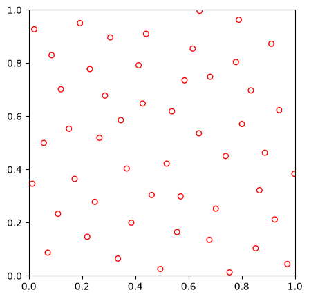
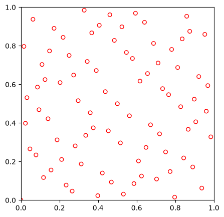
The method to be used for sampling using a different algorithm must be imported from pysampling.sample. Here, we use Latin Hypercube Sampling to generate 50 points in 2 dimensions.

from pysampling.sample import sample

X = sample("lhs", 50, 2)

Every method is reproducible via random_state, which accepts an int seed or a NumPy Generator (e.g. np.random.default_rng(1)). It draws from a local generator and never touches NumPy’s global RNG, so it is safe to call inside a larger stochastic pipeline.

To look at the results we use a small helper that draws the points in the unit square — reused for every method below so the plots are directly comparable:

import matplotlib.pyplot as plt


def show(X):
    plt.figure(figsize=(5, 5))
    plt.scatter(X[:, 0], X[:, 1], s=30, facecolors="none", edgecolors="r")
    plt.xlim(0, 1)
    plt.ylim(0, 1)
    plt.gca().set_aspect("equal")
    plt.show()


show(X)

Features

So far our library provides the following implementations:

• Random ('random')

• Latin Hypercube Sampling ('lhs')

• Sobol ('sobol')

• Halton ('halton')

• Riesz s-energy ('riesz')

The initialization of each is shown below, visualized with the show helper defined above.

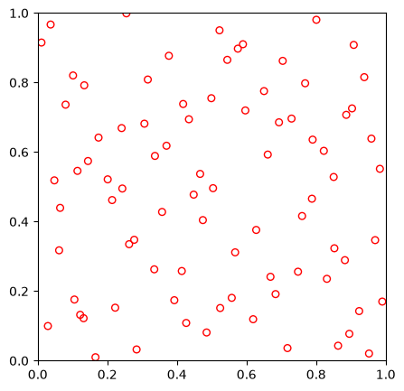
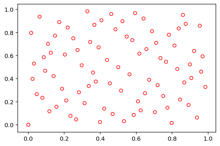
Random ('random')

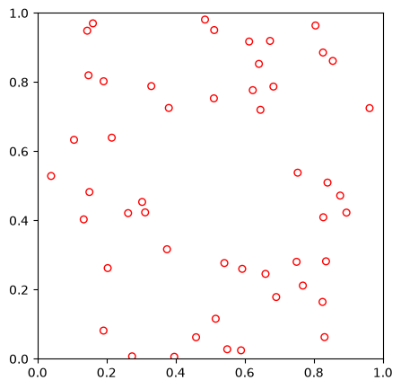
X = sample("random", 50, 2, random_state=1)
show(X)

Latin Hypercube Sampling ('lhs')

By default lhs is optimized for spacing: it runs n_iter sweeps of Morris–Mitchell within-column swap search (maximin), which keeps improving with n_iter and typically beats Sobol on both spacing and discrepancy:

X = sample("lhs", 50, 2, random_state=1)
show(X)

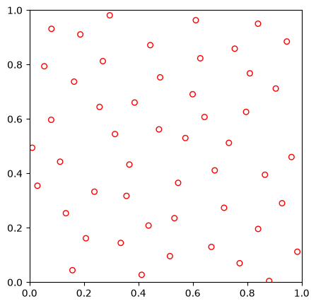
Raise n_iter for tighter spacing, or pass criterion=None for a single raw draw (fastest — already low-discrepancy, just not distance-optimized).

Keeping distance from existing points (Xp)

Xp is an existing (m, n_dim) point set that the new sample should stay away from: under the maximin criterion the minimized spacing then spans both the new points and their distance to Xp. This makes lhs an augmented / sequential design — adding infill points that avoid an existing set, e.g. earlier experiments or evaluations:

Xp = sample("lhs", 20, 2, random_state=0)        # an existing design
X = sample("lhs", 20, 2, Xp=Xp, random_state=1)  # new points avoiding Xp

plt.figure(figsize=(5, 5))
plt.scatter(Xp[:, 0], Xp[:, 1], s=40, c="0.6", label="existing (Xp)")
plt.scatter(X[:, 0], X[:, 1], s=40, facecolors="none", edgecolors="r", label="new")
plt.legend(loc="upper right")
plt.xlim(0, 1)
plt.ylim(0, 1)
plt.gca().set_aspect("equal")
plt.show()

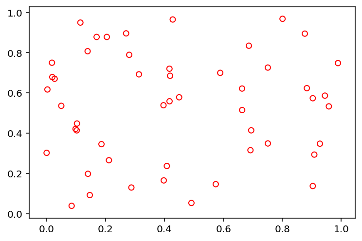
Sobol ('sobol')

X = sample("sobol", 84, 2)
show(X)

The Sobol sequence can be customized — for example, skipping the first points and leaping over points in the sequence:

X = sample("sobol", 84, 2, n_skip=100, n_leap=10)
show(X)

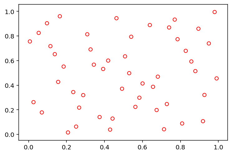
Halton ('halton')

X = sample("halton", 100, 2)
show(X)

Riesz s-energy ('riesz')

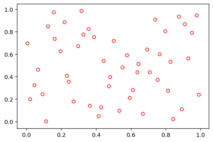
Riesz sampling places points by minimizing the s-energy sum_{i<j} 1 / ||x_i - x_j||^s — the points repel each other, so they spread out as far apart as possible. It is a maximin design: it maximizes the minimum distance between points, far more than the other methods. It is not a low-discrepancy method (and its 1-D projections collapse), so reach for sobol or lhs when uniformity or projection quality matter, and for riesz when you want maximally well-separated points.

X = sample("riesz", 100, 2, random_state=1)
show(X)

By default the energy is measured periodically — distances wrap around the unit cube (opposite faces are glued together, as on a torus), so there is no boundary for points to pile up against. Passing periodic=False instead uses ordinary Euclidean distance and clamps points into the box, which pushes them onto the boundary:

import numpy as np
import matplotlib.pyplot as plt

from pysampling.util import cdist


def min_dist(Y):
    D = cdist(Y, Y)
    np.fill_diagonal(D, np.inf)
    return D.min()


fig, axes = plt.subplots(1, 2, figsize=(10, 5))
for ax, periodic in zip(axes, [False, True]):
    Y = sample("riesz", 100, 2, random_state=1, periodic=periodic)
    ax.scatter(Y[:, 0], Y[:, 1], s=25, facecolors="none", edgecolors="r")
    ax.set_title(f"periodic={periodic}  (min-dist={min_dist(Y):.3f})")
    ax.set_xlim(0, 1)
    ax.set_ylim(0, 1)
    ax.set_aspect("equal")
plt.show()

Note — The clamped (periodic=False) variant is fine in 2-D, but it degrades as the dimension grows: almost all of a hypercube’s volume lies near its boundary, so the points collapse onto faces and corners — in 10-D nearly every coordinate ends up pinned to 0 or 1. The periodic default (recommended) avoids this and stays an even, interior-filling design. Use periodic=False only when the edges of the box are genuine hard walls.

Comparing the methods

The pysampling.measures module quantifies two complementary qualities of a design: discrepancy (how uniformly the points fill the space — lower is better) and minimum distance (how well separated they are — higher is better). These pull in different directions: low-discrepancy sequences (sobol, halton) win on uniformity, while maximin designs (riesz, and lhs with its default criterion="maxmin") win on separation.

from pysampling.measures import centered_l2_discrepancy, minimum_distance

print(f"{'method':8s} {'discrepancy ↓':>14} {'min-dist ↑':>12}")
for name in ["random", "lhs", "halton", "sobol", "riesz"]:
    Y = sample(name, 100, 2, random_state=1)
    # minimum_distance returns the negated min distance, so flip the sign
    print(f"{name:8s} {centered_l2_discrepancy(Y):>14.5f} {-minimum_distance(Y):>12.5f}")

method    discrepancy ↓   min-dist ↑
random          0.04166      0.01602
lhs             0.01020      0.06470
halton          0.02193      0.04041
sobol           0.01183      0.01105
riesz           0.01224      0.09675

Contact

Questions, bugs, or feature requests? Please open an issue on GitHub.

Maintained by Julian Blank.