pysamoo: Surrogate-Assisted Multi-objective Optimization
![]()
![]()
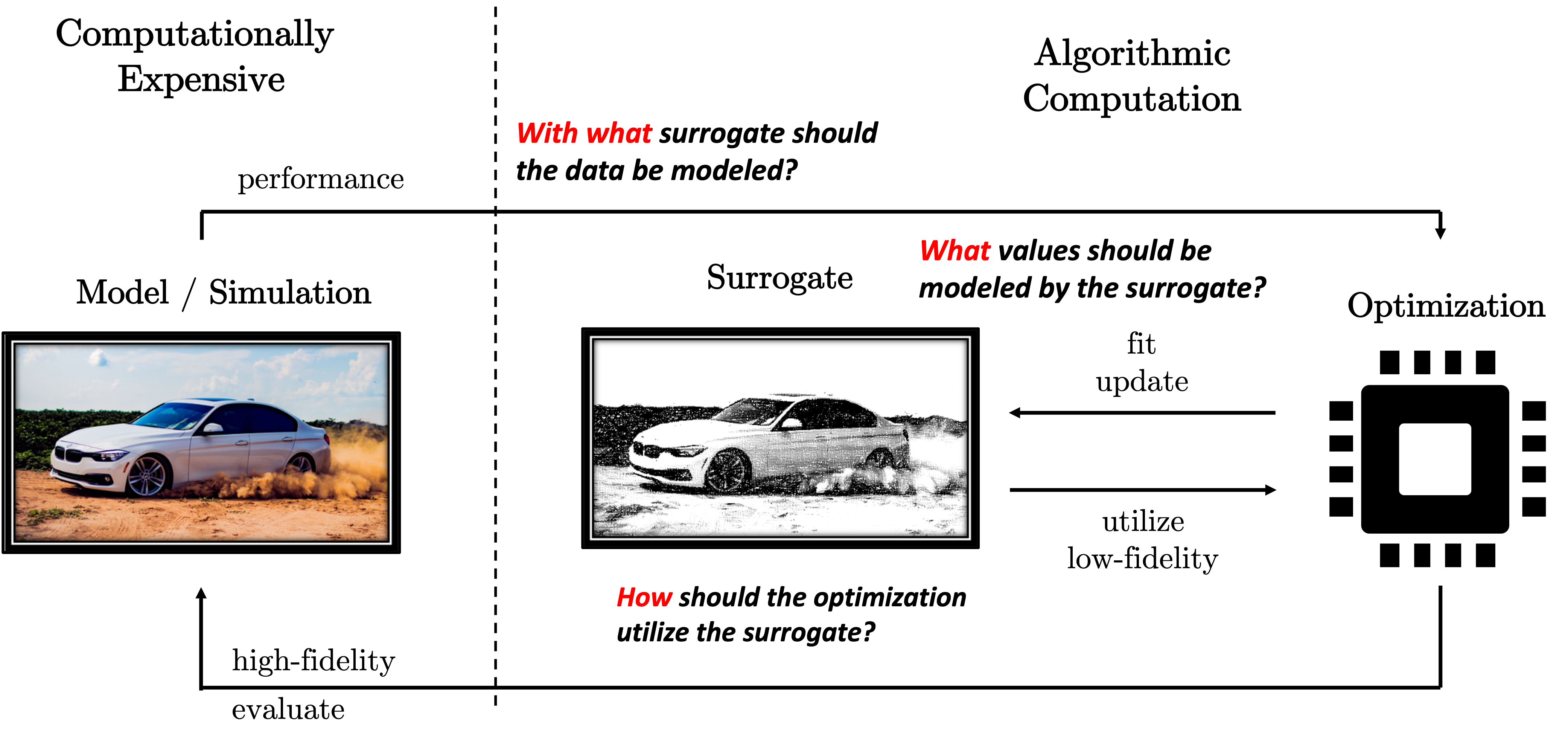
In practice, most optimization problems in practice consist of one or multiple computationally expensive objective or constraint functions to which special attention must be paid during algorithm design. Most commonly, so-called surrogates (also known as metamodels or simply approximation models) are utilized during optimization to learn from previous evaluations and exploit this knowledge in future iterations. pysamoo is an extension of pymoo - a comprehensive toolbox for multi-objective optimization - focusing on solving optimization problems with computationally expensive objective or constraint functions.
Please find the Github repository here: https://github.com/anyoptimization/pysamoo
Please find an overview of this software documentation below:
Overview
License: GNU Affero General Public License (AGPL).
Installation: How to install the current release of pysamoo.
Algorithms: An overview of algorithms and their underlying concepts.
Usage: Instructions and code snippets to execute algorithms.
Contact: Information to contact the framework’s leading developer.
Algorithm |
Framework |
multi-objective |
constrained |
Description |
None |
yes |
yes |
A simple surrogate-assisted variant of the well-known NSGA-II algorithm. |
|
PSAF |
no |
no |
An implementation using genetic algorithms assisted by surrogates. |
|
PSAF |
no |
no |
An implementation of surrogate-assisted particle swarm optimization. |
|
PSAF |
no |
no |
The popular CMAES method with surrogate assistance. |
|
GPSAF |
no |
yes |
An implementation using genetic algorithms assisted by surrogates with constrained handling |
|
GPSAF |
no |
yes |
An implementation of surrogate-assisted particle swarm optimization with constrained handling. |
|
GPSAF |
no |
no |
The popular CMAES method with surrogate assistance. |
|
GPSAF |
no |
yes |
A surrogate-assisted variant of ISRES, a well known algorithm for constrained single-objective optimization problems |
|
GPSAF |
yes |
yes |
A surrogate-assisted variant of NSGA-II, a well known algorithm for bi-objective optimization |
|
GPSAF |
yes |
yes |
An extension of GPSAF-NSGA-II for many-objective optimization problems. |
License
GNU Affero General Public License (AGPL): The GNU Affero General Public License is a modified version of the ordinary GNU GPL version 3. It has one added requirement: if you run a modified program on a server and let other users communicate with it there, your server must also allow them to download the source code corresponding to the modified version running there.
Warning
Please note that pysamoo has a more permissive software license which only allows non-commercial usage. If you intend to use pysamoo for commercial purposes please contact us.
Citation
Note
If you use this framework, we kindly ask you to cite the following paper:
@misc{pysamoo,
      title={pysamoo: Surrogate-Assisted Multi-Objective Optimization in Python},
      author={Julian Blank and Kalyanmoy Deb},
      year={2022},
      eprint={2204.05855},
      archivePrefix={arXiv},
      primaryClass={cs.NE}
}
Installation
The framework is available at the PyPi Repository and can be easily installed by:
pip install -U pysamoo
Algorithms
In this part of the software documentation, some more words about the algorithms being implemented in the framework shall be said.
Commonly, surrogates – approximation or interpolation models – are utilized during optimization to improve the convergence behavior. First, one shall distinguish between two different types of evaluations: ESEs that require to run the computationally expensive evaluation; and ASEs which is a computationally inexpensive approximation by the surrogate. Where the overall optimization run is limited by \(\texttt{ESE}^{\max}\) function evaluation, function calls of ASEs are only considered as algorithmic overhead.
Simple Surrogate Assisted (SSA)
In order to improve the convergence of NSGA-II, the surrogates provide ASEs and let the algorithm look several iterations into the future without any evaluation of ESEs. The surrogate models are used to create a set of infill solutions as follows: First, NSGA-II is run for \(k\) more iterations (starting from the best solutions found so far), returning the solution set \(X^{\texttt{(cand)}}\). The number of solutions in \(X^{\texttt{(cand)}}\) corresponds to the population size of the algorithm. After eliminating duplicates in \(X^{\texttt{(cand)}}\), the number of solutions \(N\) desired to run using ESEs needs to be selected. The selection first creates \(N\) clusters (in the objective space based on \(X^{\texttt{(cand)}}\)) using the k-means algorithm and then uses a roulette wheel selection based on the predicted crowding distances. Note that this will introduce a bias towards boundary points as they have been depicted with a crowding distance of infinity. Altogether, this results in \(N\) solutions to be then evaluated using ESEs in this optimization cycle.

PSAF
In contrast to most existing surrogate-assisted algorithms, PSAF uses not only the final solution(s) obtained by optimizing the surrogate but the whole search pattern. By making use of the search pattern, the exploration-exploitation balance is found by taking the surrogate’s accuracy into account. To allow even more flexible exploitation of the surrogate, we propose two phases. First, derive a solution set that is influenced by the surrogate, and second, introduce surrogate bias by optimizing the surrogate for a number of iterations. Both procedures are important to incorporate surrogates into existing methods effectively.
One of the major challenges when proposing a generalized optimization framework is the number and strictness of assumptions being made. On the one hand, too many assumptions restrict the applicability; on the other hand, too few assumptions limit the usage of existing elements in algorithms. In this study, we target any type of population-based algorithm with two phases in an iteration: the process of generating new solutions to be evaluated (infill) and a method processing evaluated infill solutions (advance). So, how can existing optimization methods be described into infill and advance phases? Genetic algorithms (GAs) generate new solutions using evolutionary recombination-mutation operators and then process them using an environmental survival selection operator; PSO methods create new solutions based on a particles’ current velocity, personal best, and global best, and process the solutions using a replacement strategy; CMAES samples new solutions from a normal distribution, which is then updated in each iteration. Shown by well-known state-of-the-art algorithms following or being suitable to be implemented in this optimization method design pattern, this seems to be a reasonable assumption to be made for a generic framework. Moreover, it is worth noting that some researchers and practitioners also refer to the pattern as ask-and-tell interface.

\(\alpha\)-Phase
A well-known concept in evolutionary computation to introduce a bias toward more promising solutions is tournament selection. An individual from the population has to win a tournament to contribute to the mating process. The number of competitors (\(\alpha\)) balances how greedy the selection procedure will be. On the one hand, a larger value of \(\alpha\) allows only elitist solutions to participate in mating, while a smaller value introduces less selection pressure. For genetic algorithms, the most frequently used tournament mode is the binary tournament (\(\alpha=2\)), which compares a pair of solutions regarding one or multiple metrics. A standard binary tournament implementation for constrained single-objective optimization declares the less infeasible solution as the winner if one or both solutions are infeasible or otherwise the solution with the smaller function value.
In the context of surrogate assistance, the tournament selection introduces surrogate bias during the generation of new infill solutions. Whereas in genetic algorithms, evaluated solutions (using ESE) compete with each other during mating selection, in PSAF solutions evaluated on the surrogate (ASE) are compared.

\(\beta\)-Phase
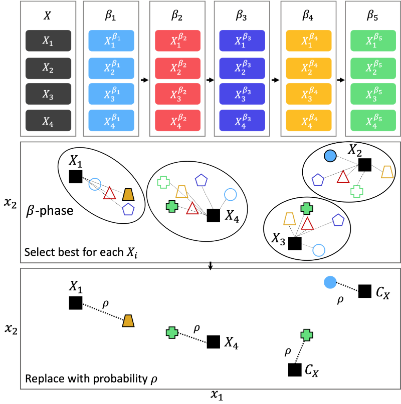
While the tournament is an effective concept to incorporate the surrogate’s approximation, it is limited by looking only a single iteration into the future. To further increase the surrogate’s impact, the baseline algorithm is continued to run for \(\beta\) more consecutive iterations on the surrogate’s approximations. Inevitably, the question of how many iterations are suitable arises and indicates the importance of tuning \(\beta\). Nevertheless, even more critical, how should the algorithm profit from simulating the algorithm on the surrogate? An inappropriate choice of \(\beta\) will cause the surrogate’s optimum to be repeatedly found and will entirely discard the baseline algorithm’s default infill procedure. This also causes a diversity loss of infill solutions and does not account for the surrogate’s approximation error. Thus, we propose a probabilistic surrogate-assisted approach that balances the surrogate’s impact on the baseline algorithm to address these issues.
An example with five iterations (\(\beta = 5\)) and four infill solutions \(X_1\), \(X_2\), \(X_3\), and \(X_4\) is also illustrated in the figure below. Calling the infill function of the baseline algorithm results in five solution sets with four solutions each. When running the algorithm, the assignment takes place, and for instance, \(X_1\) has four solutions being the closest to, and \(X_4\) has six. The assignment of the closest solution will show cluster-like arrangements and preserve diversity.
For more information please we would like to the corresponding publication:
Publication:
BibTex:
@inproceedings{10.1145/3449639.3459297,
author = {Blank, Julian and Deb, Kalyanmoy},
title = {PSAF: A Probabilistic Surrogate-Assisted Framework for Single-Objective Optimization},
year = {2021},
isbn = {9781450383509},
publisher = {Association for Computing Machinery},
address = {New York, NY, USA},
url = {https://doi.org/10.1145/3449639.3459297},
doi = {10.1145/3449639.3459297},
booktitle = {Proceedings of the Genetic and Evolutionary Computation Conference},
pages = {652–659},
numpages = {8},
keywords = {simulation optimization, metamodel-based optimization, surrogate-assisted optimization, genetic algorithms, evolutionary computing},
location = {Lille, France},
series = {GECCO '21}
}
GPSAF
Next, PSAF shall be extended to be suitable to handle multiple objectives and constraints. GPSAF follows the two-phase concept as PSAF. However, the \(\alpha\)-phase and the \(\beta\)-phase now have to consider multiple criteria when comparing solutions.
Extension of PSAF to constrained and multi-objective optimization
What needs to be modified?
Multiple Surrogates: One for each constraint, one for each objective
Solution Comparisons: Instead of comparing only the objective, the constraint satisfaction and Pareto Dominance now need to be considered.
Exploration vs. Exploitation: The bottle variable rho needs to be redefined.
For single-objective optimization, the \(\alpha\)-phase has already been described. There, the comparison of the two solutions is based only on one single objective value. For the more generic version with constrainAnalogously to PSAF, GPSAF further increases the surrogate’s impact by looking \(\beta\) iterations into the future through calling infill and advance of the baseline algorithm repetitively. To obtain the \(\beta\)-solution for constrained multi-objective problems, we use a so-called Probabilistic Knockout Tournament (PKT) to select solutions from each cluster with the goal of self-adaptively exploiting surrogates. The goal is to use surrogates more when they provide accurate predictions but use them more carefully when they provide only rough estimations. Necessary for generalization, PKT also applies to problems with multiple objectives and constraints, often with varying complexities and surrogate errors to be considered.ts and objectives, the winner of each solution pool is determined as follows: if all solutions are infeasible, select the least infeasible solution; otherwise, select a non-dominated solution (break ties randomly). For both the constraint and objective values, only ASEs are used. Otherwise, the \(\alpha\)-phase remains the same, including its responsibilities and mechanics.
Analogously to PSAF, GPSAF further increases the surrogate’s impact by looking \(\beta\) iterations into the future through calling infill and advance of the baseline algorithm repetitively. To obtain the \(\beta\)-solution for constrained multi-objective problems, we use a so-called PKT to select solutions from each cluster with the goal of self-adaptively exploiting surrogates. The goal is to use surrogates more when they provide accurate predictions but use them more carefully when they provide only rough estimations. Necessary for generalization, PKT also applies to problems with multiple objectives and constraints, often with varying complexities and surrogate errors to be considered.

For more information please we would like to the corresponding publication:
Publication:
BibTex:
@misc{gpsaf,
  doi = {10.48550/ARXIV.2204.04054},
  url = {https://arxiv.org/abs/2204.04054},
  author = {Blank, Julian and Deb, Kalyanmoy},
  keywords = {Optimization and Control (math.OC), Machine Learning (cs.LG), Mathematical Software (cs.MS), FOS: Mathematics, FOS: Mathematics, FOS: Computer and information sciences, FOS: Computer and information sciences, G.1.6; G.1.2; I.6.3, 68U07},
  title = {GPSAF: A Generalized Probabilistic Surrogate-Assisted Framework for Constrained Single- and Multi-objective Optimization},
  publisher = {arXiv},
  year = {2022},
  copyright = {arXiv.org perpetual, non-exclusive license}
}
Usage
In general, pysamoo uses the main functionalities of pymoo for defining the optimization problem. However, it provides a new set of algorithms designed for computationally expensive functions.
SSA-NSGA-II
For bi-objective optimization problems, a variant of NSGA-II called Simple Surrogate Assisted NSGA-II (SSA-NSGA-II) could be a good starting point.
[1]:
from pymoo.optimize import minimize
from pymoo.problems.multi.zdt import ZDT1
from pymoo.visualization.scatter import Scatter
from pysamoo.algorithms.ssansga2 import SSANSGA2
problem = ZDT1(n_var=10)
algorithm = SSANSGA2(n_initial_doe=50,
n_infills=10,
surr_pop_size=100,
surr_n_gen=50)
res = minimize(
problem,
algorithm,
('n_evals', 200),
seed=1,
verbose=True)
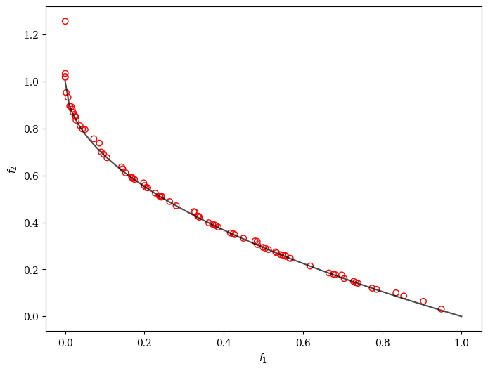
plot = Scatter()
plot.add(problem.pareto_front(), plot_type="line", color="black", alpha=0.7)
plot.add(res.F, facecolor="none", edgecolor="red")
plot.show()
==========================================================================
n_gen  |  n_eval  | n_nds  |      igd      |       gd      |       hv
==========================================================================
     1 |       50 |      8 |  1.5264428232 |  2.2537834613 |  0.000000E+00
     2 |       60 |     12 |  0.0447088272 |  0.5062280434 |  0.6033429744
     3 |       70 |     20 |  0.0317166787 |  0.1679151161 |  0.6185749342
     4 |       80 |     24 |  0.0254483220 |  0.0084090160 |  0.6309981786
     5 |       90 |     29 |  0.0230370295 |  0.0144214557 |  0.6344052194
     6 |      100 |     35 |  0.0212245222 |  0.0132708565 |  0.6370941415
     7 |      110 |     42 |  0.0195966238 |  0.0130647742 |  0.6396760863
     8 |      120 |     48 |  0.0177374193 |  0.0108200540 |  0.6420831108
     9 |      130 |     50 |  0.0175224609 |  0.0174397893 |  0.6422432439
    10 |      140 |     53 |  0.0158996130 |  0.0094427526 |  0.6444796025
    11 |      150 |     59 |  0.0153706224 |  0.0176365671 |  0.6454315717
    12 |      160 |     63 |  0.0138676188 |  0.0168468611 |  0.6472923167
    13 |      170 |     69 |  0.0136776440 |  0.0160061467 |  0.6478761757
    14 |      180 |     74 |  0.0125680488 |  0.0153520648 |  0.6495825568
    15 |      190 |     79 |  0.0121553028 |  0.0148969083 |  0.6500744968
    16 |      200 |     83 |  0.0114381989 |  0.0104171897 |  0.6513000952
[1]:
<pymoo.visualization.scatter.Scatter at 0x1606d9cd0>
PSAF-GA
[2]:
from pymoo.algorithms.soo.nonconvex.ga import GA
from pymoo.optimize import minimize
from pymoo.problems.single import Ackley
from pysamoo.algorithms.psaf import PSAF

problem = Ackley(n_var=10)

algorithm = GA(pop_size=20, n_offsprings=10)

algorithm = PSAF(algorithm, n_initial_doe=30, alpha=10, beta=30, max_rho=0.7, n_max_infills=10, n_max_doe=500)

res = minimize(
    problem,
    algorithm,
    ('n_evals', 300),
    seed=2,
    verbose=True)

print("Best solution found: \nX = %s\nF = %s\nCV=%s" % (res.X, res.F, res.CV))
================================================================================================================================================================
n_gen  |  n_eval  |     f_min     |     f_gap     |       r2      |      bias     |      mae      |                            model
================================================================================================================================================================
     1 |       30 |  2.036794E+01 |  2.036794E+01 |             - |             - |  0.2738756231 |             RBF[kernel=linear,tail=constant,normalized=True]
     2 |       40 |  1.614481E+01 |  1.614481E+01 |  0.3763933967 |  0.7000000000 |  0.5348634440 |     RBF[kernel=cubic,tail=linear+quadratic,normalized=False]
     3 |       50 |  1.614481E+01 |  1.614481E+01 |  0.3976668792 |  0.7000000000 |  0.6351592863 |             RBF[kernel=linear,tail=constant,normalized=True]
     4 |       60 |  1.479848E+01 |  1.479848E+01 |  0.2795887538 |  0.7000000000 |  0.8588945004 |        RBF[kernel=mq,tail=linear+quadratic,normalized=False]
     5 |       70 |  1.310293E+01 |  1.310293E+01 | -2.495997E-01 |  0.7000000000 |  1.0450900866 |    RBF[kernel=linear,tail=linear+quadratic,normalized=False]
     6 |       80 |  1.268252E+01 |  1.268252E+01 |  0.1339056137 |  0.7000000000 |  1.4391106360 |             RBF[kernel=linear,tail=constant,normalized=True]
     7 |       90 |  1.198853E+01 |  1.198853E+01 |  0.1004963738 |  0.7000000000 |  1.1109921715 |                                                     krg-cont
     8 |      100 |  1.070961E+01 |  1.070961E+01 | -1.356016E-01 |  0.7000000000 |  1.1038348109 |                                                     krg-cont
     9 |      110 |  9.0245380210 |  9.0245380210 | -3.871513E-02 |  0.7000000000 |  1.1543317740 |                                                     krg-cont
    10 |      120 |  8.8940807360 |  8.8940807360 | -3.268868E-02 |  0.7000000000 |  0.8929508896 |                                                     krg-cont
    11 |      130 |  8.4131436015 |  8.4131436015 |  0.1006854678 |  0.7000000000 |  0.9085243047 |                                                     krg-cont
    12 |      140 |  7.8246574061 |  7.8246574061 | -8.313746E-01 |  0.7000000000 |  0.5755873561 |                                                      krg-lin
    13 |      150 |  7.0834789444 |  7.0834789444 |  0.4176491944 |  0.7000000000 |  0.6266697638 |                                                     krg-cont
    14 |      160 |  6.0646712483 |  6.0646712483 |  0.2139484322 |  0.7000000000 |  0.4735844314 |                                                      krg-lin
    15 |      170 |  5.9366538601 |  5.9366538601 |  0.4389178038 |  0.7000000000 |  0.5479664682 |                                                      krg-lin
    16 |      180 |  5.6660865834 |  5.6660865834 |  0.0852439643 |  0.7000000000 |  0.5417697700 |                                                     krg-cont
    17 |      190 |  5.0408470264 |  5.0408470264 | -1.175129E-01 |  0.7000000000 |  0.5883136752 |                                                     krg-cont
    18 |      200 |  4.6010645765 |  4.6010645765 | -6.175937E-01 |  0.7000000000 |  0.5818244380 |                                                     krg-cont
    19 |      210 |  4.5254801853 |  4.5254801853 | -1.176425E+00 |  0.7000000000 |  0.6073626579 |                                                     krg-cont
    20 |      220 |  3.9720804105 |  3.9720804105 | -2.661123E+00 |  0.7000000000 |  0.5095595451 |                                                     krg-cont
    21 |      230 |  3.9720804105 |  3.9720804105 | -2.542042E+00 |  0.7000000000 |  0.5437289305 |                                                     krg-cont
    22 |      240 |  3.6608112233 |  3.6608112233 | -2.833233E+00 |  0.7000000000 |  0.4527138832 |                                                     krg-cont
    23 |      250 |  3.4490801784 |  3.4490801784 | -2.355759E+00 |  0.7000000000 |  0.4256093867 |                                                      krg-lin
    24 |      260 |  3.0871007367 |  3.0871007367 | -4.493002E+00 |  0.7000000000 |  0.5288772233 |                                                      krg-lin
    25 |      270 |  3.0871007367 |  3.0871007367 | -5.774866E+00 |  0.7000000000 |  0.6508483015 |                                                      krg-lin
    26 |      280 |  3.0020921309 |  3.0020921309 | -9.136042E+00 |  0.7000000000 |  0.5603836037 |                                                      krg-lin
    27 |      290 |  2.9161694816 |  2.9161694816 | -8.368297E+00 |  0.7000000000 |  0.6311346722 |                                                      krg-lin
    28 |      300 |  2.8268436055 |  2.8268436055 | -1.130324E+01 |  0.7000000000 |  0.6046665921 |                                                      krg-lin
Best solution found:
X = [ 0.97346909  0.03114564 -1.06840523  0.04009389 -0.0521602   0.27861872
  1.03606787 -0.07359098 -0.98842002 -0.03037685]
F = [2.82684361]
CV=[0.]
PSAF-DE
[3]:
from pymoo.algorithms.soo.nonconvex.de import DE
from pymoo.optimize import minimize
from pymoo.problems.single import Ackley
from pysamoo.algorithms.psaf import PSAF

problem = Ackley(n_var=10)

algorithm = DE(pop_size=20, n_offsprings=10)

algorithm = PSAF(algorithm, n_initial_doe=30, alpha=10, beta=30, max_rho=0.7, n_max_infills=10, n_max_doe=500)

res = minimize(
    problem,
    algorithm,
    ('n_evals', 300),
    seed=2,
    verbose=True)

print("Best solution found: \nX = %s\nF = %s\nCV=%s" % (res.X, res.F, res.CV))
================================================================================================================================================================
n_gen  |  n_eval  |     f_min     |     f_gap     |       r2      |      bias     |      mae      |                            model
================================================================================================================================================================
     1 |       30 |  2.036794E+01 |  2.036794E+01 |             - |             - |  0.2738756231 |             RBF[kernel=linear,tail=constant,normalized=True]
     2 |       40 |  1.647220E+01 |  1.647220E+01 |  0.3763933967 |  0.7000000000 |  0.6182901894 |     RBF[kernel=cubic,tail=linear+quadratic,normalized=False]
     3 |       50 |  1.647220E+01 |  1.647220E+01 |  0.3341034259 |  0.7000000000 |  1.0337146201 |               RBF[kernel=linear,tail=linear,normalized=True]
     4 |       60 |  1.647220E+01 |  1.647220E+01 | -2.325472E-01 |  0.7000000000 |  1.1952242311 |               RBF[kernel=linear,tail=linear,normalized=True]
     5 |       70 |  1.526461E+01 |  1.526461E+01 | -2.483244E-01 |  0.7000000000 |  1.3548503486 |               RBF[kernel=linear,tail=linear,normalized=True]
     6 |       80 |  1.353941E+01 |  1.353941E+01 | -2.854016E-01 |  0.7000000000 |  1.7725365031 |                RBF[kernel=mq,tail=constant,normalized=False]
     7 |       90 |  1.353941E+01 |  1.353941E+01 | -6.876366E-01 |  0.7000000000 |  0.4617090285 |                                                     krg-cont
     8 |      100 |  1.013393E+01 |  1.013393E+01 |  0.9168512037 |  0.9168512037 |  0.5703039705 |                                                     krg-cont
     9 |      110 |  1.013393E+01 |  1.013393E+01 |  0.8668379853 |  0.8668379853 |  0.5693628726 |                                                      krg-lin
    10 |      120 |  9.7623502147 |  9.7623502147 |  0.8575626049 |  0.8575626049 |  0.5840720180 |                                                      krg-lin
    11 |      130 |  9.0558961856 |  9.0558961856 |  0.8603199816 |  0.8603199816 |  0.5523672725 |                                                      krg-lin
    12 |      140 |  9.0558961856 |  9.0558961856 |  0.8717525585 |  0.8717525585 |  0.5662209881 |                                                     krg-cont
    13 |      150 |  9.0237677371 |  9.0237677371 |  0.7948496762 |  0.7948496762 |  0.4791068868 |                                                     krg-cont
    14 |      160 |  6.6233913732 |  6.6233913732 |  0.7726556864 |  0.7726556864 |  0.4877162796 |                                                     krg-cont
    15 |      170 |  6.6233913732 |  6.6233913732 |  0.8429714787 |  0.8429714787 |  0.4170345533 |                                                     krg-cont
    16 |      180 |  5.7617523828 |  5.7617523828 |  0.8788722441 |  0.8788722441 |  0.4330862204 |                                                     krg-cont
    17 |      190 |  5.7617523828 |  5.7617523828 |  0.8581799389 |  0.8581799389 |  0.4180912931 |                                                      krg-lin
    18 |      200 |  3.9941402749 |  3.9941402749 |  0.8439598319 |  0.8439598319 |  0.3781019454 |                                                      krg-lin
    19 |      210 |  3.9941402749 |  3.9941402749 |  0.9041705189 |  0.9041705189 |  0.4175998236 |                                                      krg-lin
    20 |      220 |  3.9914565327 |  3.9914565327 |  0.8239454481 |  0.8239454481 |  0.4864284914 |                                                     krg-cont
    21 |      230 |  3.9914565327 |  3.9914565327 |  0.8487160611 |  0.8487160611 |  0.4507227421 |                                                     krg-cont
    22 |      240 |  3.8211595495 |  3.8211595495 |  0.8687656158 |  0.8687656158 |  0.5130797895 |                                                     krg-cont
    23 |      250 |  3.6463534058 |  3.6463534058 |  0.8626187728 |  0.8626187728 |  0.5621053352 |                                                     krg-cont
    24 |      260 |  3.6463534058 |  3.6463534058 |  0.8201204070 |  0.8201204070 |  0.5304724523 |                                                     krg-cont
    25 |      270 |  3.6463534058 |  3.6463534058 |  0.8196879465 |  0.8196879465 |  0.5066856628 |                                                     krg-cont
    26 |      280 |  3.6463534058 |  3.6463534058 |  0.7784551445 |  0.7784551445 |  0.5778498499 |                                                     krg-cont
    27 |      290 |  3.6463534058 |  3.6463534058 |  0.7348469218 |  0.7348469218 |  0.5360693341 |                                                      krg-lin
    28 |      300 |  3.6463534058 |  3.6463534058 |  0.7136844062 |  0.7136844062 |  0.5894129213 |                                                      krg-lin
Best solution found:
X = [-0.017365   -0.13750357 -0.05619225  0.369787   -0.54064667  0.02531361
  0.18193453  1.34091596 -0.55839746 -0.31890217]
F = [3.64635341]
CV=[0.]
PSAF-CMAES
[4]:
from pymoo.algorithms.soo.nonconvex.cmaes import SimpleCMAES
from pymoo.optimize import minimize
from pymoo.problems.single import Ackley
from pysamoo.algorithms.psaf import PSAF

problem = Ackley(n_var=10)

algorithm = SimpleCMAES(pop_size=20)

algorithm = PSAF(algorithm, n_initial_doe=30, alpha=10, beta=30, max_rho=0.7, n_max_infills=10, n_max_doe=500)

res = minimize(
    problem,
    algorithm,
    ('n_evals', 300),
    seed=2,
    verbose=True)

print("Best solution found: \nX = %s\nF = %s\nCV=%s" % (res.X, res.F, res.CV))
================================================================================================================================================================
n_gen  |  n_eval  |     f_min     |     f_gap     |       r2      |      bias     |      mae      |                            model
================================================================================================================================================================
     1 |       30 |  2.036794E+01 |  2.036794E+01 |             - |             - |  0.2738756231 |             RBF[kernel=linear,tail=constant,normalized=True]
     2 |       40 |  1.332973E+01 |  1.332973E+01 |  0.3763933967 |  0.7000000000 |  0.7291380548 |     RBF[kernel=cubic,tail=linear+quadratic,normalized=False]
     3 |       50 |  1.332973E+01 |  1.332973E+01 |  0.2592841419 |  0.7000000000 |  0.9917695888 |        RBF[kernel=mq,tail=linear+quadratic,normalized=False]
     4 |       60 |  1.332973E+01 |  1.332973E+01 |  0.1644667959 |  0.7000000000 |  1.1552330246 |               RBF[kernel=linear,tail=linear,normalized=True]
     5 |       70 |  1.332973E+01 |  1.332973E+01 |  0.3694414291 |  0.7000000000 |  1.5138747301 |               RBF[kernel=linear,tail=linear,normalized=True]
     6 |       80 |  1.332973E+01 |  1.332973E+01 |  0.2600993833 |  0.7000000000 |  1.8085470200 |               RBF[kernel=linear,tail=linear,normalized=True]
     7 |       90 |  1.241845E+01 |  1.241845E+01 |  0.2038351057 |  0.7000000000 |  0.6335623668 |                                                     krg-cont
     8 |      100 |  7.3256172613 |  7.3256172613 |  0.8492853728 |  0.8492853728 |  0.8690919422 |                                                     krg-cont
     9 |      110 |  7.3256172613 |  7.3256172613 |  0.7486633888 |  0.7486633888 |  1.0053520252 |                                                     krg-cont
    10 |      120 |  6.9655651500 |  6.9655651500 |  0.6028752305 |  0.7000000000 |  1.1338932661 |                                                     krg-cont
    11 |      130 |  5.0841360021 |  5.0841360021 |  0.6039414826 |  0.7000000000 |  1.1598374455 |                                                     krg-cont
    12 |      140 |  5.0841360021 |  5.0841360021 |  0.6085190250 |  0.7000000000 |  1.2980426541 |                                                     krg-cont
    13 |      150 |  4.7082954697 |  4.7082954697 |  0.6037349339 |  0.7000000000 |  1.0560636000 |                                                     krg-cont
    14 |      160 |  3.9307717509 |  3.9307717509 |  0.6416580369 |  0.7000000000 |  0.8196459781 |                                                     krg-cont
    15 |      170 |  3.9307717509 |  3.9307717509 |  0.7689568545 |  0.7689568545 |  0.6934795741 |                                                     krg-cont
    16 |      180 |  3.6005443620 |  3.6005443620 |  0.7947301965 |  0.7947301965 |  0.6828921049 |                                                     krg-cont
    17 |      190 |  3.5337383218 |  3.5337383218 |  0.7862944244 |  0.7862944244 |  0.5887485674 |                                                      krg-lin
    18 |      200 |  3.5337383218 |  3.5337383218 |  0.8054350086 |  0.8054350086 |  0.8994223086 |                                                      krg-lin
    19 |      210 |  3.5337383218 |  3.5337383218 |  0.2592954046 |  0.7000000000 |  0.9427215928 |                                                      krg-lin
    20 |      220 |  3.5337383218 |  3.5337383218 |  0.0777094174 |  0.7000000000 |  1.0415795870 |                                                      krg-lin
    21 |      230 |  3.5337383218 |  3.5337383218 | -2.692331E-01 |  0.7000000000 |  1.0218187624 |                                                      krg-lin
    22 |      240 |  3.5337383218 |  3.5337383218 | -7.771233E-01 |  0.7000000000 |  1.1893524253 |                                                      krg-lin
    23 |      250 |  2.9110175231 |  2.9110175231 | -1.132129E+00 |  0.7000000000 |  0.8852039354 |                                                     krg-cont
    24 |      260 |  2.6880983494 |  2.6880983494 | -1.270011E+00 |  0.7000000000 |  1.0067140755 |                                                     krg-cont
    25 |      270 |  2.6880983494 |  2.6880983494 | -2.820539E+00 |  0.7000000000 |  1.0239253459 |                                                     krg-cont
    26 |      280 |  2.6880983494 |  2.6880983494 | -3.069151E+00 |  0.7000000000 |  1.0617400742 |                                                      krg-lin
    27 |      290 |  2.6260580244 |  2.6260580244 | -3.561686E+00 |  0.7000000000 |  0.9515962802 |                                                      krg-lin
    28 |      300 |  2.6260580244 |  2.6260580244 | -4.387418E+00 |  0.7000000000 |  1.3332084142 |              RBF[kernel=cubic,tail=constant,normalized=True]
Best solution found:
X = [-0.05580694 -0.09378573 -0.37298884 -0.08638338  0.0515077  -0.41373204
  0.09691779  1.07067447  0.1263253  -0.20414152]
F = [2.62605802]
CV=[0.]
GPSAF-GA
[5]:
from pymoo.algorithms.soo.nonconvex.ga import GA
from pymoo.optimize import minimize
from pymoo.problems.single import Ackley
from pysamoo.algorithms.gpsaf import GPSAF

problem = Ackley(n_var=10)

algorithm = GA(pop_size=20, n_offsprings=10)

algorithm = GPSAF(algorithm, n_initial_doe=30, alpha=10, beta=30, n_max_infills=10, n_max_doe=500)

res = minimize(
    problem,
    algorithm,
    ('n_evals', 300),
    seed=2,
    verbose=True)

print("Best solution found: \nX = %s\nF = %s\nCV=%s" % (res.X, res.F, res.CV))
================================================================================================================================================
n_gen  |  n_eval  |     f_min     |     f_gap     |  n_influenced |      mae      |                            model
================================================================================================================================================
     1 |       30 |  2.036794E+01 |  2.036794E+01 |             - |  0.2395537352 |          RBF[kernel=gaussian,tail=quadratic,normalized=True]
     2 |       40 |  9.6180845318 |  9.6180845318 |          4/10 |  0.7292616206 |         RBF[kernel=gaussian,tail=quadratic,normalized=False]
     3 |       50 |  9.5397702619 |  9.5397702619 |          4/10 |  1.2838259268 |         RBF[kernel=gaussian,tail=quadratic,normalized=False]
     4 |       60 |  8.3350419429 |  8.3350419429 |          5/10 |  1.1933475702 |   RBF[kernel=gaussian,tail=linear+quadratic,normalized=True]
     5 |       70 |  8.2371788716 |  8.2371788716 |          4/10 |  1.1919714473 |   RBF[kernel=gaussian,tail=linear+quadratic,normalized=True]
     6 |       80 |  8.0191285291 |  8.0191285291 |          2/10 |  0.8810109187 |                                            kriging-const-ARD
     7 |       90 |  7.8519168526 |  7.8519168526 |          4/10 |  0.7338034351 |                                                  kriging-lin
     8 |      100 |  7.7553809035 |  7.7553809035 |          2/10 |  0.7521845637 |                                                  kriging-lin
     9 |      110 |  7.3837499736 |  7.3837499736 |          6/10 |  0.8561025281 |                                                  kriging-lin
    10 |      120 |  7.3837499736 |  7.3837499736 |          6/10 |  2.7239305748 |                                                kriging-quadr
    11 |      130 |  7.3837499736 |  7.3837499736 |          4/10 |  1.7610057486 |                                                  kriging-lin
    12 |      140 |  7.3640055044 |  7.3640055044 |          6/10 |  1.0600526491 |                                            kriging-const-ARD
    13 |      150 |  7.0657745472 |  7.0657745472 |          4/10 |  1.2643272170 |                                            kriging-const-ARD
    14 |      160 |  7.0657745472 |  7.0657745472 |          6/10 |  2.2759640477 |                                                  kriging-lin
    15 |      170 |  7.0407792334 |  7.0407792334 |          3/10 |  2.1436566074 |                                                  kriging-lin
    16 |      180 |  6.9854628698 |  6.9854628698 |          4/10 |  0.3210627737 |                                                kriging-quadr
    17 |      190 |  6.9847040068 |  6.9847040068 |          2/10 |  1.8313479569 |                                                  kriging-lin
    18 |      200 |  6.9162278041 |  6.9162278041 |          3/10 |  1.2739195852 |                                                  kriging-lin
    19 |      210 |  6.9081087618 |  6.9081087618 |          3/10 |  0.6008899786 |                                                  kriging-lin
    20 |      220 |  6.8826264252 |  6.8826264252 |          6/10 |  0.6377193155 |                                                  kriging-lin
    21 |      230 |  6.8815544475 |  6.8815544475 |          5/10 |  0.6552357623 |                                                  kriging-lin
    22 |      240 |  6.8403116305 |  6.8403116305 |          6/10 |  0.0724192352 |                                                kriging-quadr
    23 |      250 |  6.8274044511 |  6.8274044511 |          3/10 |  0.4952315643 |                                                  kriging-lin
    24 |      260 |  6.8274035650 |  6.8274035650 |          7/10 |  0.5406026626 |                                                  kriging-lin
    25 |      270 |  6.8030346170 |  6.8030346170 |          5/10 |  0.4775624871 |                                                  kriging-lin
    26 |      280 |  6.8009722666 |  6.8009722666 |          1/10 |  0.4409766638 |                                                  kriging-lin
    27 |      290 |  5.2446639674 |  5.2446639674 |          4/10 |  1.043396E+01 |                                                  kriging-lin
    28 |      300 |  5.1590950227 |  5.1590950227 |          2/10 |  1.336450E+01 |                                                kriging-quadr
Best solution found:
X = [-2.00803163  1.86061669 -2.09794872  1.95560802 -0.14461223  0.08631508
  0.07473123 -0.07630844  0.89663685 -0.25277987]
F = [5.15909502]
CV=[0.]
GPSAF-DE
[6]:
from pymoo.algorithms.soo.nonconvex.de import DE
from pymoo.optimize import minimize
from pymoo.problems.single import Ackley
from pysamoo.algorithms.gpsaf import GPSAF

problem = Ackley(n_var=10)

algorithm = DE(pop_size=20, n_offsprings=10)

algorithm = GPSAF(algorithm, n_initial_doe=30, alpha=10, beta=30, n_max_infills=10, n_max_doe=500)

res = minimize(
    problem,
    algorithm,
    ('n_evals', 300),
    seed=1,
    verbose=True)

print("Best solution found: \nX = %s\nF = %s\nCV=%s" % (res.X, res.F, res.CV))
================================================================================================================================================
n_gen  |  n_eval  |     f_min     |     f_gap     |  n_influenced |      mae      |                            model
================================================================================================================================================
     1 |       30 |  2.033913E+01 |  2.033913E+01 |             - |  0.2584492905 |                   RBF[kernel=mq,tail=linear,normalized=True]
     2 |       40 |  1.489029E+01 |  1.489029E+01 |          5/10 |  0.4320034794 |                   RBF[kernel=mq,tail=linear,normalized=True]
     3 |       50 |  1.489029E+01 |  1.489029E+01 |          6/10 |  0.5599724717 |               RBF[kernel=linear,tail=linear,normalized=True]
     4 |       60 |  1.203982E+01 |  1.203982E+01 |          8/10 |  0.7991257442 |               RBF[kernel=linear,tail=linear,normalized=True]
     5 |       70 |  1.203982E+01 |  1.203982E+01 |          5/10 |  0.8959677659 |             RBF[kernel=linear,tail=constant,normalized=True]
     6 |       80 |  1.203982E+01 |  1.203982E+01 |          5/10 |  1.0550719580 |             RBF[kernel=linear,tail=constant,normalized=True]
     7 |       90 |  1.190403E+01 |  1.190403E+01 |          4/10 |  0.6643174886 |                                                kriging-const
     8 |      100 |  8.7732279452 |  8.7732279452 |          7/10 |  0.7612524061 |                                                kriging-const
     9 |      110 |  8.7732279452 |  8.7732279452 |          6/10 |  0.6504482134 |                                                kriging-const
    10 |      120 |  8.7732279452 |  8.7732279452 |          7/10 |  0.6183165691 |                                                kriging-const
    11 |      130 |  7.4950684256 |  7.4950684256 |          8/10 |  0.6255644662 |                                                kriging-const
    12 |      140 |  7.4950684256 |  7.4950684256 |          7/10 |  0.6872365051 |                                                kriging-const
BIASED: TOO CLOSE (SKIP)
    13 |      150 |  7.4950684256 |  7.4950684256 |          8/10 |  0.5375685411 |                                                kriging-const
    14 |      160 |  6.4510590085 |  6.4510590085 |          4/10 |  0.4939197965 |                                            kriging-const-ARD
    15 |      170 |  5.9600945536 |  5.9600945536 |          7/10 |  0.4638647655 |                                                kriging-quadr
    16 |      180 |  5.9600945536 |  5.9600945536 |          7/10 |  0.4446192503 |                                            kriging-const-ARD
    17 |      190 |  5.4886456424 |  5.4886456424 |          7/10 |  0.4839298024 |                                            kriging-const-ARD
    18 |      200 |  5.4886456424 |  5.4886456424 |          9/10 |  0.6993539907 |                                              kriging-lin-ARD
    19 |      210 |  5.4886456424 |  5.4886456424 |          6/10 |  0.7372165210 |                                              kriging-lin-ARD
    20 |      220 |  5.4886456424 |  5.4886456424 |          8/10 |  0.7630410210 |                                              kriging-lin-ARD
    21 |      230 |  5.4886456424 |  5.4886456424 |          7/10 |  0.6797742577 |                                            kriging-quadr-ARD
    22 |      240 |  5.2455941969 |  5.2455941969 |          5/10 |  0.7468197492 |                                              kriging-lin-ARD
    23 |      250 |  3.8890189117 |  3.8890189117 |          5/10 |  0.5426021921 |                                              kriging-lin-ARD
    24 |      260 |  3.8890189117 |  3.8890189117 |          3/10 |  0.4366853768 |                                              kriging-lin-ARD
    25 |      270 |  3.8890189117 |  3.8890189117 |          5/10 |  0.3746281150 |                                            kriging-const-ARD
    26 |      280 |  3.8890189117 |  3.8890189117 |          7/10 |  0.4238507263 |                                            kriging-const-ARD
    27 |      290 |  3.8890189117 |  3.8890189117 |          5/10 |  0.3439499037 |                                            kriging-quadr-ARD
    28 |      300 |  3.8890189117 |  3.8890189117 |          4/10 |  0.5077978046 |                                            kriging-const-ARD
Best solution found:
X = [-0.73853388  0.20019719  0.29418694 -0.68726892  0.33516822  0.03035722
 -0.48582207 -0.93401104  0.81073807 -0.38538059]
F = [3.88901891]
CV=[0.]
GPSAF-ISRES
[7]:
from pymoo.algorithms.soo.nonconvex.isres import ISRES
from pymoo.problems import get_problem
from pymoo.optimize import minimize
from pysamoo.algorithms.gpsaf import GPSAF

problem = get_problem("g1")

algorithm = ISRES()

algorithm = GPSAF(algorithm,
                  alpha=3,
                  beta=30,
                  n_max_infills=1)

res = minimize(
    problem,
    algorithm,
    ('n_evals', 50),
    seed=1,
    verbose=True)

print("Best solution found: \nX = %s\nF = %s\nCV=%s" % (res.X, res.F, res.CV))
=================================================================================================
n_gen  |  n_eval  |     cv_min    |     cv_avg    |     f_min     |     f_gap     |  n_influenced
=================================================================================================
     1 |       27 |  1.714499E+02 |  5.617944E+02 |             - |             - |             -
     2 |       28 |  1.7247367719 |  5.617944E+02 |             - |             - |           1/1
     3 |       29 |  0.000000E+00 |  5.617944E+02 | -6.400043E+00 |  8.5999570206 |           1/1
     4 |       30 |  0.000000E+00 |  5.617944E+02 | -1.079833E+01 |  4.2016695983 |           1/1
     5 |       31 |  0.000000E+00 |  5.617944E+02 | -1.155193E+01 |  3.4480660762 |           1/1
     6 |       32 |  0.000000E+00 |  5.617944E+02 | -1.304470E+01 |  1.9552979195 |           1/1
     7 |       33 |  0.000000E+00 |  5.617944E+02 | -1.454634E+01 |  0.4536595946 |           1/1
     8 |       34 |  0.000000E+00 |  5.617944E+02 | -1.480047E+01 |  0.1995280575 |           1/1
     9 |       35 |  0.000000E+00 |  5.617944E+02 | -1.491833E+01 |  0.0816667392 |           1/1
    10 |       36 |  0.000000E+00 |  5.617944E+02 | -1.495020E+01 |  0.0498020785 |           1/1
    11 |       37 |  0.000000E+00 |  5.617944E+02 | -1.497953E+01 |  0.0204729495 |           1/1
    12 |       38 |  0.000000E+00 |  5.617944E+02 | -1.498599E+01 |  0.0140111011 |           1/1
    13 |       39 |  0.000000E+00 |  5.617944E+02 | -1.499666E+01 |  0.0033414569 |           1/1
    14 |       40 |  0.000000E+00 |  5.617944E+02 | -1.499798E+01 |  0.0020232532 |           1/1
    15 |       41 |  0.000000E+00 |  5.617944E+02 | -1.499893E+01 |  0.0010657277 |           1/1
    16 |       42 |  0.000000E+00 |  5.617944E+02 | -1.499951E+01 |  0.0004923939 |           1/1
    17 |       43 |  0.000000E+00 |  5.617944E+02 | -1.499989E+01 |  0.0001121181 |           1/1
    18 |       44 |  0.000000E+00 |  5.617944E+02 | -1.499996E+01 |  0.0000392967 |           1/1
    19 |       45 |  0.000000E+00 |  5.617944E+02 | -1.499998E+01 |  0.0000213215 |           1/1
    20 |       46 |  0.000000E+00 |  5.617944E+02 | -1.499999E+01 |  6.450720E-06 |           1/1
    21 |       47 |  0.000000E+00 |  5.617944E+02 | -1.500000E+01 |  2.063368E-06 |           1/1
    22 |       48 |  0.000000E+00 |  5.617944E+02 | -1.500000E+01 |  1.004444E-06 |           1/1
    23 |       49 |  0.000000E+00 |  5.617944E+02 | -1.500000E+01 |  7.880460E-07 |           1/1
    24 |       50 |  0.000000E+00 |  5.617944E+02 | -1.500000E+01 |  3.512184E-07 |           1/1
Best solution found:
X = [0.99999999 1.         1.         0.99999999 0.99999996 0.99999999
 0.99999999 0.99999999 1.         2.99999992 2.99999995 2.99999995
 1.        ]
F = [-14.99999965]
CV=[0.]
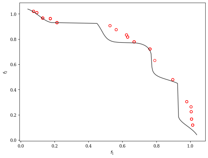
GPSAF-NSGA-II
[8]:
import numpy as np
from pymoo.algorithms.moo.nsga2 import NSGA2
from pymoo.optimize import minimize
from pymoo.problems.multi import ZDT1
from pymoo.visualization.scatter import Scatter
from pysamoo.algorithms.gpsaf import GPSAF
problem = ZDT1(n_var=10)
algorithm = NSGA2(pop_size=20, n_offsprings=10)
algorithm = GPSAF(algorithm,
alpha=10,
beta=50,
n_max_doe=100,
n_max_infills=np.inf,
)
res = minimize(
problem,
algorithm,
('n_evals', 250),
seed=1,
verbose=True)
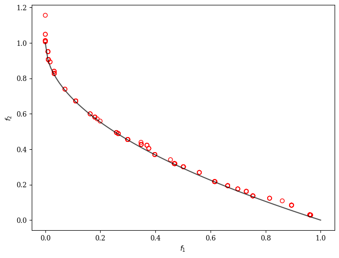
plot = Scatter()
plot.add(problem.pareto_front(), plot_type="line", color="black", alpha=0.7)
plot.add(res.F, facecolor="none", edgecolor="red")
plot.show()
==========================================================================================================================
n_gen  |  n_eval  | n_nds  |      igd      |       gd      |       hv      |  n_influenced |     mae f1    |     mae f2
==========================================================================================================================
     1 |       21 |      3 |  1.8942829534 |  3.0095912826 |  0.000000E+00 |             - |  2.158343E-16 |  0.1648489778
     2 |       31 |      3 |  0.4620001734 |  0.7493117302 |  0.1510010190 |          4/10 |  2.875825E-16 |  0.1602687910
     3 |       41 |      2 |  0.3371490822 |  0.2924047767 |  0.3268413114 |          2/10 |  3.001494E-16 |  0.1174748180
     4 |       51 |      8 |  0.1408073065 |  0.2210541972 |  0.4390090282 |          4/10 |  3.452678E-16 |  0.0959817810
     5 |       61 |     10 |  0.1408073065 |  0.0554779978 |  0.4390090282 |          2/10 |  3.650537E-16 |  0.0920210809
     6 |       71 |     16 |  0.1221342838 |  0.0449904710 |  0.4557288877 |          4/10 |  4.895776E-16 |  0.0935525354
     7 |       81 |     27 |  0.0827579407 |  0.0468689921 |  0.5246360468 |          4/10 |  4.549254E-16 |  0.0804396406
     8 |       91 |     43 |  0.0665862375 |  0.0457088275 |  0.5597220040 |          5/10 |  5.034923E-16 |  0.0734327256
     9 |      101 |     47 |  0.0619377292 |  0.0447108249 |  0.5713835331 |          5/10 |  4.815151E-16 |  0.0677243980
    10 |      111 |     61 |  0.0388290475 |  0.0363894044 |  0.6033660247 |          8/10 |  5.531123E-16 |  0.0557135910
    11 |      121 |     66 |  0.0346932634 |  0.0310968683 |  0.6118625353 |          6/10 |  5.023857E-16 |  0.0514084161
    12 |      131 |     71 |  0.0289701336 |  0.0298619940 |  0.6199182144 |          6/10 |  6.586745E-16 |  0.0580864746
    13 |      141 |     80 |  0.0259409226 |  0.0264607872 |  0.6244944372 |          5/10 |  6.353598E-16 |  0.0663689181
    14 |      151 |     90 |  0.0250694448 |  0.0228440028 |  0.6262433378 |          5/10 |  5.765809E-16 |  0.0502260611
    15 |      161 |     99 |  0.0244332270 |  0.0232342003 |  0.6281135848 |          8/10 |  5.182270E-16 |  0.0512215780
    16 |      171 |    106 |  0.0242365158 |  0.0192595759 |  0.6285037545 |          8/10 |  3.970392E-16 |  0.0534405466
    17 |      181 |    107 |  0.0223183843 |  0.0149311969 |  0.6310924941 |          3/10 |  5.725975E-16 |  0.0440707098
    18 |      191 |    123 |  0.0218602416 |  0.0143220756 |  0.6318522249 |          6/10 |  8.820722E-16 |  0.0486144418
    19 |      201 |    138 |  0.0211919510 |  0.0138804874 |  0.6332318400 |          6/10 |  1.540363E-15 |  0.0497609611
    20 |      211 |    155 |  0.0211090608 |  0.0133719333 |  0.6333551695 |          6/10 |  1.865587E-15 |  0.0442893928
    21 |      221 |    166 |  0.0203041406 |  0.0127681633 |  0.6344643397 |          8/10 |  1.988264E-15 |  0.0582482969
    22 |      231 |    171 |  0.0200470557 |  0.0120744782 |  0.6352276331 |          5/10 |  2.353805E-15 |  0.0773347096
    23 |      241 |    173 |  0.0199378688 |  0.0113533889 |  0.6358860735 |          5/10 |  2.550337E-15 |  0.0800614458
    24 |      251 |    192 |  0.0196526487 |  0.0121477068 |  0.6363797924 |          9/10 |  3.551637E-15 |  0.0640281394
[8]:
<pymoo.visualization.scatter.Scatter at 0x103c25850>
GPSAF-NSGA-III
[9]:
import numpy as np

from pymoo.algorithms.moo.nsga3 import NSGA3
from pymoo.problems import get_problem
from pymoo.util.ref_dirs import get_reference_directions
from pymoo.optimize import minimize
from pymoo.problems.multi import TNK
from pymoo.visualization.scatter import Scatter
from pysamoo.algorithms.gpsaf import GPSAF

problem = TNK()

ref_dirs = get_reference_directions("das-dennis", 2, n_points=20)

# create the algorithm object
algorithm = NSGA3(pop_size=20,
                  n_offsprings=10,
                  ref_dirs=ref_dirs)


algorithm = GPSAF(algorithm,
                  alpha=10,
                  beta=50,
                  n_max_doe=100,
                  )

res = minimize(
    problem,
    algorithm,
    ('n_evals', 200),
    seed=1,
    verbose=True)

plot = Scatter()
plot.add(problem.pareto_front(), plot_type="line", color="black", alpha=0.7)
plot.add(res.F, facecolor="none", edgecolor="red")
plot.show()
==========================================================================================================================
n_gen  |  n_eval  | n_nds  |     cv_min    |     cv_avg    |      igd      |       gd      |       hv      |  n_influenced
==========================================================================================================================
     1 |        5 |      1 |  0.5717037305 |  7.3349018351 |             - |             - |             - |             -
     2 |       15 |      2 |  0.000000E+00 |  7.3349018351 |  0.2653544470 |  0.0984902580 |  0.0294105975 |          7/10
     3 |       25 |      6 |  0.000000E+00 |  7.3349018351 |  0.1688552083 |  0.1110745959 |  0.0804323054 |          6/10
     4 |       35 |     12 |  0.000000E+00 |  7.3349018351 |  0.1626975751 |  0.1069272188 |  0.0812678935 |          4/10
     5 |       45 |     16 |  0.000000E+00 |  7.3349018351 |  0.1626975751 |  0.1074034919 |  0.0812678935 |          2/10
     6 |       55 |      7 |  0.000000E+00 |  7.3349018351 |  0.1568291260 |  0.0536053149 |  0.1334154871 |          4/10
     7 |       65 |      9 |  0.000000E+00 |  7.3349018351 |  0.1448912306 |  0.0645102339 |  0.1336500488 |          4/10
     8 |       75 |     13 |  0.000000E+00 |  7.3349018351 |  0.1197962927 |  0.0676481356 |  0.1552136458 |          7/10
     9 |       85 |     16 |  0.000000E+00 |  7.3349018351 |  0.1197962927 |  0.0687271946 |  0.1552136458 |          1/10
    10 |       95 |     21 |  0.000000E+00 |  7.3349018351 |  0.0893101188 |  0.0667513661 |  0.1983892329 |          9/10
    11 |      105 |     26 |  0.000000E+00 |  7.3349018351 |  0.0594609081 |  0.0484714727 |  0.2116452805 |          7/10
    12 |      115 |     36 |  0.000000E+00 |  7.3349018351 |  0.0573628701 |  0.0455119835 |  0.2254828364 |          8/10
    13 |      125 |     45 |  0.000000E+00 |  7.3349018351 |  0.0571111062 |  0.0453376673 |  0.2258291227 |          5/10
    14 |      135 |     59 |  0.000000E+00 |  7.3349018351 |  0.0555906801 |  0.0455882251 |  0.2316224246 |          6/10
    15 |      145 |     72 |  0.000000E+00 |  7.3349018351 |  0.0555906801 |  0.0462793825 |  0.2316224246 |          4/10
    16 |      155 |     81 |  0.000000E+00 |  7.3349018351 |  0.0550140152 |  0.0473746175 |  0.2332016113 |          9/10
    17 |      165 |     90 |  0.000000E+00 |  7.3349018351 |  0.0545351583 |  0.0479898213 |  0.2335873099 |          6/10
    18 |      175 |    102 |  0.000000E+00 |  7.3349018351 |  0.0544481014 |  0.0472218443 |  0.2338235521 |          9/10
    19 |      185 |     95 |  0.000000E+00 |  7.3349018351 |  0.0508618111 |  0.0389046008 |  0.2379154517 |          9/10
    20 |      195 |     92 |  0.000000E+00 |  7.3349018351 |  0.0498523756 |  0.0336684226 |  0.2382643368 |          5/10
    21 |      205 |    103 |  0.000000E+00 |  7.3349018351 |  0.0495946407 |  0.0339564545 |  0.2388966697 |          2/10
[9]:
<pymoo.visualization.scatter.Scatter at 0x161313f10>
Tools
Constrained Sampling for Design of Experiments (DOE)
For more information and more context, please see the following publication:
@InProceedings{10.1007/978-3-030-72062-9_21,
author="Blank, Julian
and Deb, Kalyanmoy",
editor="Ishibuchi, Hisao
and Zhang, Qingfu
and Cheng, Ran
and Li, Ke
and Li, Hui
and Wang, Handing
and Zhou, Aimin",
title="Constrained Bi-objective Surrogate-Assisted Optimization of Problems with Heterogeneous Evaluation Times: Expensive Objectives and Inexpensive Constraints",
booktitle="Evolutionary Multi-Criterion Optimization",
year="2021",
publisher="Springer International Publishing",
address="Cham",
pages="257--269",
isbn="978-3-030-72062-9"
}
Let us say our goal is to find 50 feasible designs for the SRN problem. We assume that the constraints are computationally inexpensive in contrast to the objectives requiring a time-consuming evaluation.
[10]:
from pymoo.problems.multi import SRN
problem = SRN()

n_points = 50
The function returning the constrained violation (CV) given a design can then be implemented by:
[11]:
def calc_cv(X):
    G = problem.evaluate(X, return_values_of=["G"])
    return np.maximum(G, 0.0).sum(axis=1)
Now let us define a plot function showing the design space and show infeasible solutions in red and feasible ones in blue:
[12]:
import matplotlib.pyplot as plt

def plot(X):

    xl, xu = problem.bounds()

    def circle(x=0, y=0, r=1):
        theta = np.linspace(0, 2 * np.pi, 100)
        return x + r * np.cos(theta), y + r * np.sin(theta)


    fig, ax = plt.subplots(figsize=(6, 6))

    feas = calc_cv(X) <= 0

    ax.scatter(X[feas, 0], X[feas, 1], s=30, facecolors='none', edgecolors='blue')
    ax.scatter(X[~feas, 0], X[~feas, 1], s=30, facecolors='none', edgecolors='red')

    x, y = circle(r=15)
    ax.plot(x, y, color="black", alpha=0.6)

    x = np.linspace(-20, 20)
    y = 1 / 3 * x + 10 / 3
    ax.plot(x, y, color="black", alpha=0.6)

    ax.set_aspect(1)

    ax.set_xlim(xl[0], xu[0])
    ax.set_ylim(xl[1], xu[1])

    ax.set_xlabel("$x_1$")
    ax.set_ylabel("$x_2$")

    plt.show()
If we perform LHS sampling, the result might look as follows:
[13]:
from pymoo.operators.sampling.lhs import LHS

X = LHS().do(problem, n_points).get("X")
plot(X)
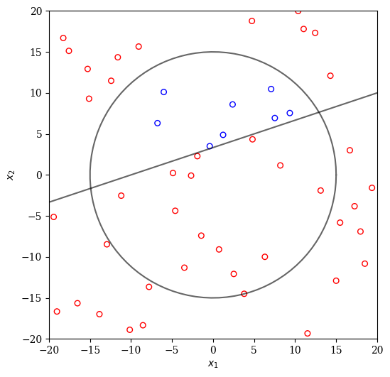
Clearly, the majority of designs are infeasible. A simple improvement of this method is repeating the sampling multiple times now until the required number of points has been found.
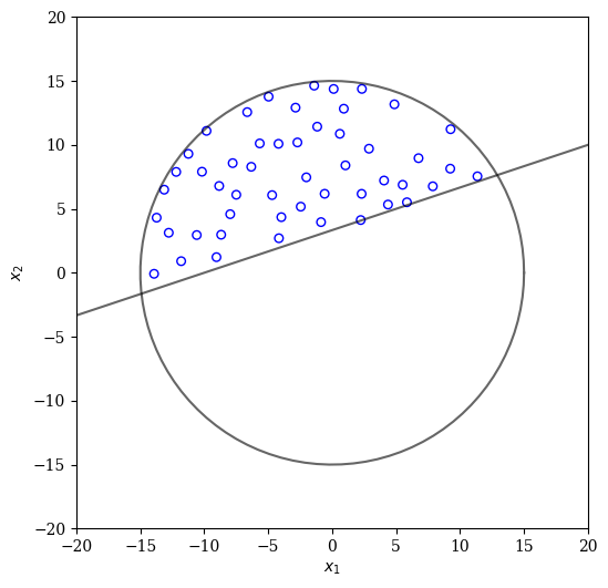
[14]:
from pysamoo.sampling.rejection import RejectionConstrainedSampling

X = RejectionConstrainedSampling(calc_cv).do(problem, n_points).get("X")
plot(X)
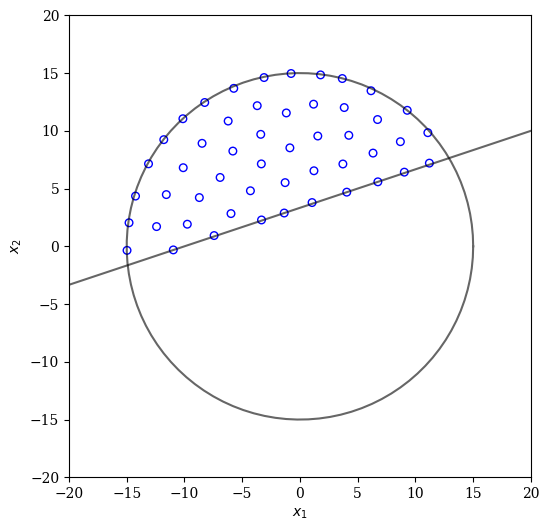
By using a more sophisticated energy-based approach the uniformity can be further improved:
[15]:
from pysamoo.sampling.energy import EnergyConstrainedSampling

X = EnergyConstrainedSampling(calc_cv).do(problem, n_points).get("X")
plot(X)
Contact
Feel free to contact us if you have any question:
Julian Blank (blankjul [at] msu.edu)
Michigan State University
Computational Optimization and Innovation Laboratory (COIN)
East Lansing, MI 48824, USA